
Has anything like this ever happened to you?
- A type of fish you used to eat years ago is harder to come by and more expensive
- Your garden used to thrive, but now it’s being destroyed by a new insect
- You don’t see the flora and fauna you used to and instead are seeing large abundances of one or two new species
It might not seem like it, but these stories are likely the impacts of a poor resource management decision. Ecosystems are composed of an extremely complicated web of plants, animals, microscopic organisms, fungi, people, precipitation, and so much more. When the abundance of one component changes, the rest of the ecosystem reacts to those changes. This is a very normal, even healthy, characteristic of ecosystems, as they need to be resilient to natural changes in weather patterns, migration behaviors, etc. However, when we as humans leave too heavy of a mark on an ecosystem, it can often create unforeseen changes that are more negative than we anticipated.

Predicting the future and learning from the past
Land managers play a delicate and sometimes impossible game when they manipulate ecosystems. They are operating to optimize an ecosystem’s health especially in relation to human impacts. Much thought needs to go into any decision in order to reduce and prepare for any negative, unintended consequences. Much of their work involves predicting the future by asking questions such as:
- What happens if I increase hunter permits?
- What happens if there’s a drought?
- What happens if this insect goes extinct?
In order to make better predictions around land management decisions, it’s also important to learn from the past. Studying how past actions or inactions have altered ecosystems can inform the decisions land managers make on the same or similar ecosystems in the future. They might approach learning from the past by asking questions such as:
- What might have caused the eradication of elk in this ecosystem?
- Why did coyotes suffer when grassland restoration efforts increased?
- What impacts did that forest fire have on this ecosystem?
Scientists Dean Pearson, T.J. Clark-Wolf, Beau Larkin, and Philip Ramsey recognize how tricky land management decisions can be and have developed a published qualitative model that allows you to model an ecosystem. Subsequently, MPG Ranch has been working to make this impressive model more accessible to larger audiences. They’ve enlisted Stamen’s expertise in solving thorny technical problems to create the MPG Matrix. The app allows anyone to manipulate and experiment with a pre-built modeled ecosystem, also known as a matrix, or even build their own matrix from scratch.
Modeling an ecosystem
It would be exhausting and ultimately unproductive to include every one of the thousands of organisms present in an ecosystem in your matrix. Instead, matrices attempt to capture the key players in an ecosystem. Each player is added to an ecosystem as a “node,” which can be seen on the main page of a matrix as small boxes that display the name, picture, and abundance of that player. Nodes are bucketed into trophic levels, depending on where they operates in the food chain.
Nodes are assigned settings such as name, trophic level, average abundances, and population criteria as noted by how they exist in the ecosystem. Each node is also given a series of connections, depending on which nodes they impact or are impacted by. These connections can be viewed by hovering on a node and following the arrows in the connections panel on the right side of the screen. Arrows leading away from a highlighted node indicate players that are impacted by that node. Arrows leading back to a highlighted node indicate which players impact that node. Negative and positive interactions are indicated by a red and blue arrow, respectively, with the interaction strength denoted on a scale from 0–1.
Creating a matrix requires much trial and error as it is a delicate balance of node settings and inter-node connections. MPG Ranch has set up a gallery of public matrices which are the best place to start when familiarizing yourself with the simulation. From there, you can follow along their resources to create experiments from an existing matrix and new matrices all together.
Case study: MPG Grasslands
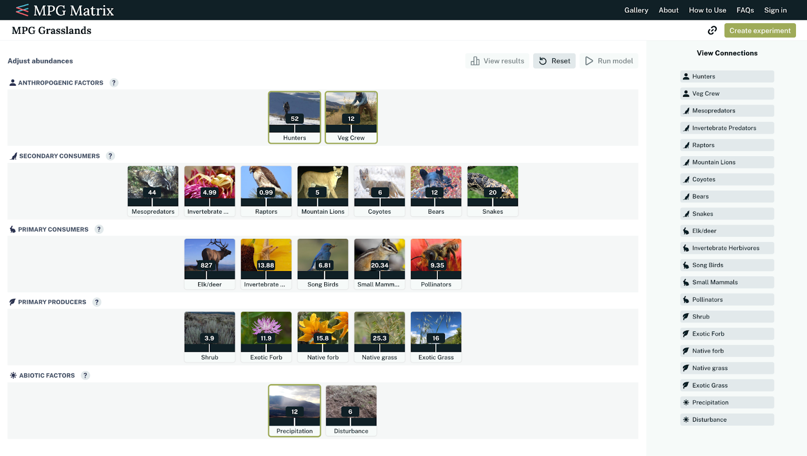
Let’s imagine a land manager wants to see how hunting elk and deer could impact other species indirectly using the public matrix MPG Grasslands. As you can see above, there are five different trophic levels to bucket the nodes in this ecosystem:
- Anthropogenic factors: Human actions that influence ecosystems such as harvesting plants or animals (e.g., timber harvest or fishing), adding pollutants or nutrients to a system, providing food or water subsidy to a system, controlling fire, etc.
- Secondary consumers: Organisms, usually predators or parasites, that consume animal tissue to build and sustain their populations.
- Primary consumers: Organisms such as herbivores that consume plant tissue to build and sustain their populations.
- Primary producers: Organisms like plants and certain bacteria and cyanobacteria that can produce organic compounds from solar or chemical energy sources by way of photosynthesis or chemosynthesis.
- Abiotic factors: Non-living components of ecosystems such as nutrients, water, solar or chemical energy that provide the basic elements for life.
Each node is denoted by its name, image, and relative abundance. The abundance units vary depending on the type of node, but in this case you can see how there are more hunters than vegetation crew in the ecosystem, 52 vs. 12, respectively.
By hovering on the nodes in the connections panel or trophic level buckets, you can see how hunters negatively impact only elk/deer. On the other hand, Elk/deer impacts and are impacted by almost half of the other nodes in the ecosystem. This means that any change to hunters in the ecosystem impacts elk/deer, which in turn impacts many other nodes as the change ripples throughout the ecosystem.
Infinite play in the ecosystem sandbox
When the nodes seem to be operating properly as you’ve found the right settings, it’s time to start playing in your ecosystem sandbox. Whenever a change is made to a matrix, the model that powers each matrix “runs” hundreds of times until it achieves an equilibrium, or balance, in the ecosystem. The final node abundances depend on the defined starting node abundances and connections.
Every node is set as an input or output which defines how it will operate within the model. Inputs (signified in the matrix by a green outline) have fixed abundances and will not react to other nodes when the model is run and changes are made to the system. Inputs are generally nodes whose abundances are set as experimental by the user or abiotic factors that should not react to the rest of the changes in the ecosystem.
Once inputs are set, you can go in and test how changing the input abundances impacts the rest of the ecosystem by moving the abundance sliders around. At any point, you can add new inputs, but keep in mind that inputs should usually make up less than 10% of the nodes in a matrix. Setting too many fixed abundances typically can add too many variables to run effective experiments.
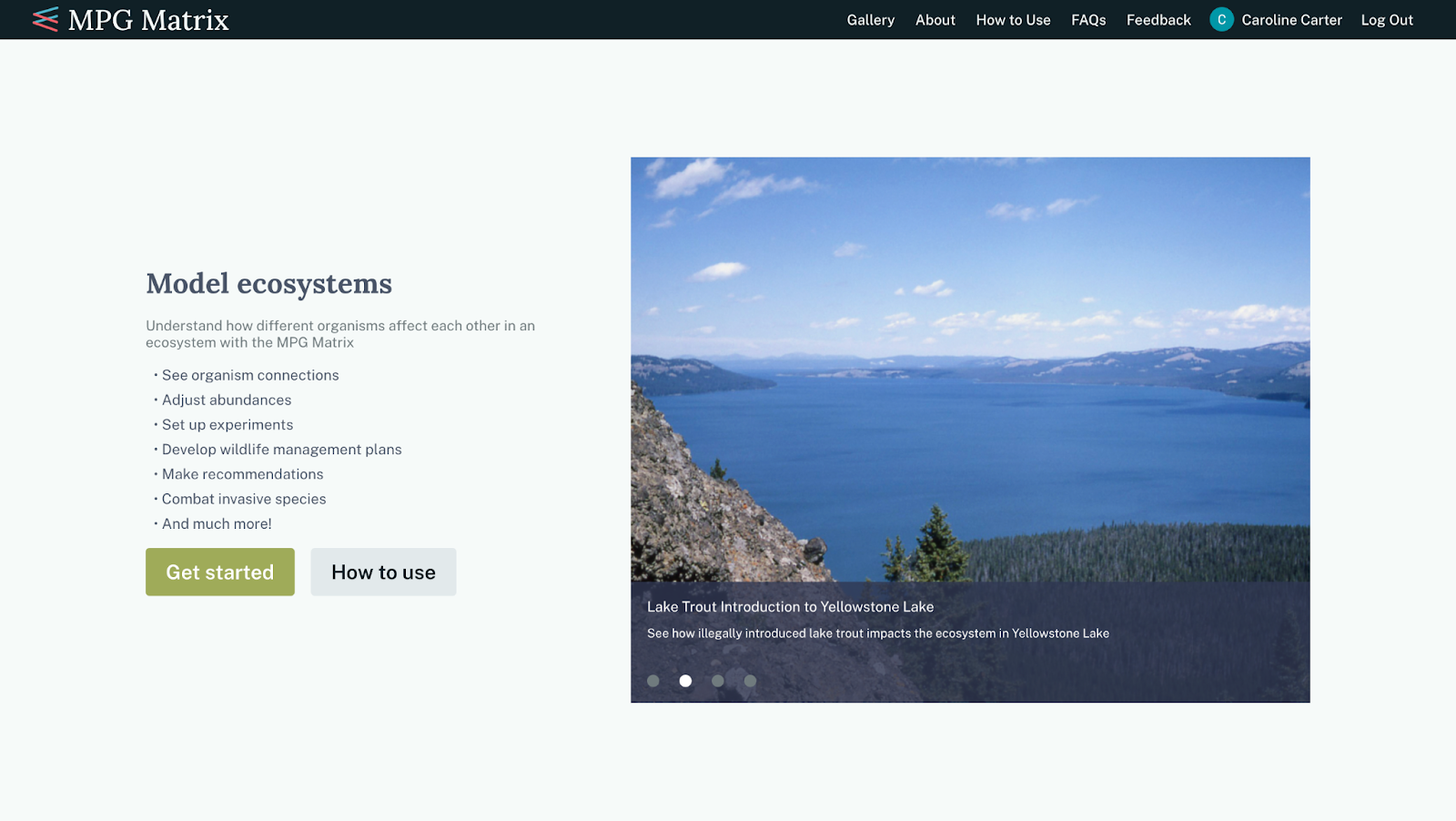
Case study: Lake trout introduction to Yellowstone Lake
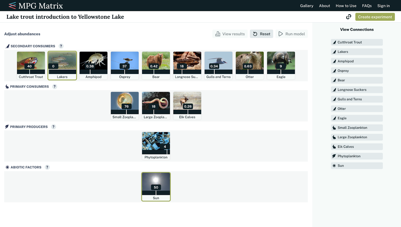
Let’s imagine a land manager wants to see what happens if they were to re-introduce lake trout to Yellowstone Lake using the public matrix Lake trout introduction to Yellowstone Lake. With lakers as an input in the matrix, as denoted by its green outline, they can increase the abundance to see what impacts that has on the rest of the system. In this example, note how the sun is also an input because the amount of sunshine should not change depending on any other change in the ecosystem.

Each node has a draggable abundance slider. If we move the lakers abundance from 0 to 200 and select “Run model,” we can watch the impacts trickle down. Note how when the user is interacting with lakers, they see its connections in the connections panel on the right hand side. Thus, we would expect that changing lakers would have an impact on cutthroat trout, amphipod, longnose suckers, small zooplankton, and large zooplankton. However, when we run the model, we can see how changing the abundance of lakers impacts almost every node in the ecosystem because lakers have indirection connections with almost every node.
Now, let’s reset the system and drag the lakers abundance to 1000 instead of 200 as noted above. We can see that it impacts the same nodes but significantly more. Increasing the amount of lakers added to the system by five times has much larger impacts on the abundances of the rest of the nodes.
If we wanted to get an even closer look at our results, we can select “View results” to see what changed. We can see that the node that was impacted the most was cutthroat trout, which makes sense as it was the strongest connection for lakers. It is likely that these two species compete for food, so increasing the amount of lakers by 1000 ultimately caused a local extinction of cutthroat trout. The node impacted the second most was the osprey, which is quite interesting as lakers do not have a direct connection to ospreys in this matrix. It is likely that ospreys prey on other nodes that decreased in abundance due to the introduction of 1000 lakers to the ecosystem.
The MPG Matrix allows for us to get a more complete picture of an ecosystem and the complexities of the possible effects of actions or inactions. By setting up the web of connections, we can see firsthand how quickly changes ripple out to almost every node in an ecosystem. For example, in our lakers example, three of the five nodes that were impacted the most had no direct connections to lakers.
Expanding to broader audiences
While we discussed this tool with respect to land managers, they are only a slice of the user base for the MPG Matrix. There is an entire library of education modules for middle and high school students learning about ecological concepts. College and graduate students as well as even researchers set up their own ecosystems to study and manipulate in the MPG Matrix. The goal of the MPG Matrix is to continue to learn about the complex inner workings of ecological systems and to carry on making it more accessible to less technical audiences. Stay tuned in the following months for even more improvements!

We at Stamen have loved working on visualizing this fascinating data model, as we really needed to get to know both the model and the user base to create something impactful. If you have data needing to be visualized related to ecology, land management, or anything else, please drop us a line!