
As cartographers, we want to make beautiful maps that grab our readers’ attention. Sometimes we wish our maps could jump out of the screen or off the page, and with a recent trend in cartography we’re starting to see more and more maps that seem to do just that.
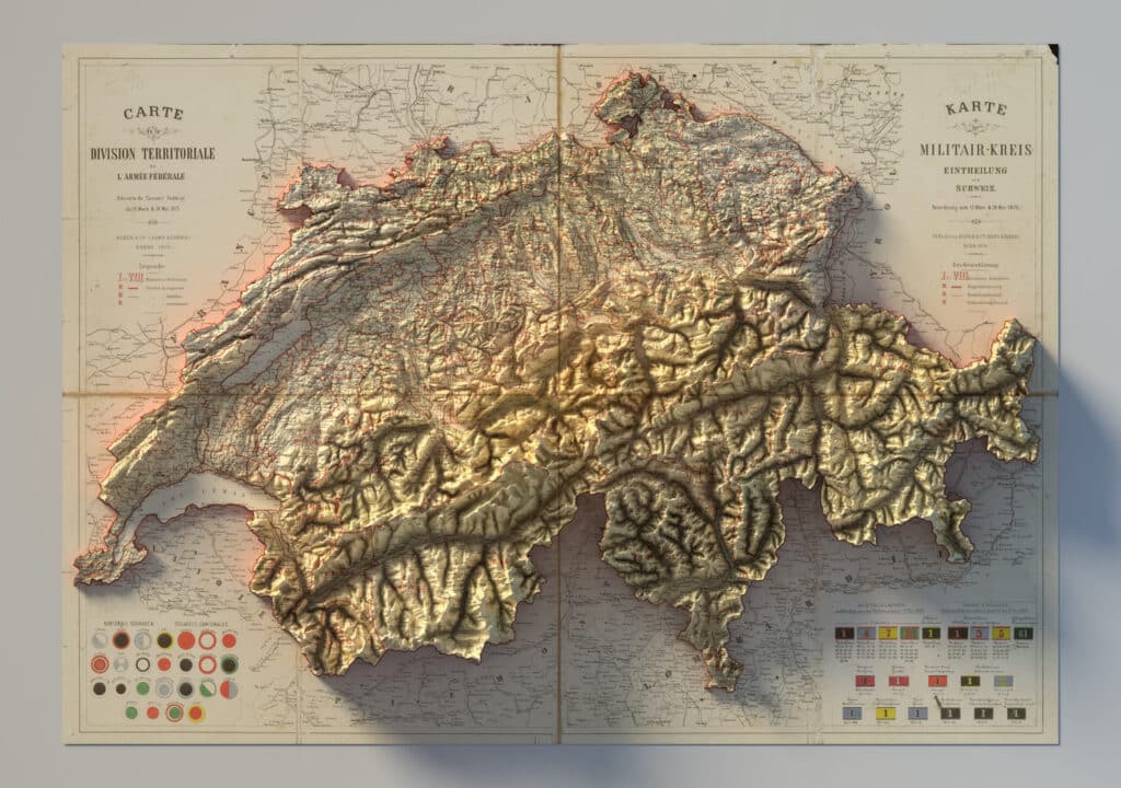
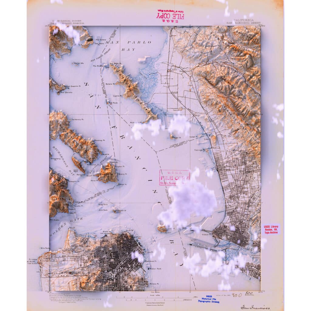
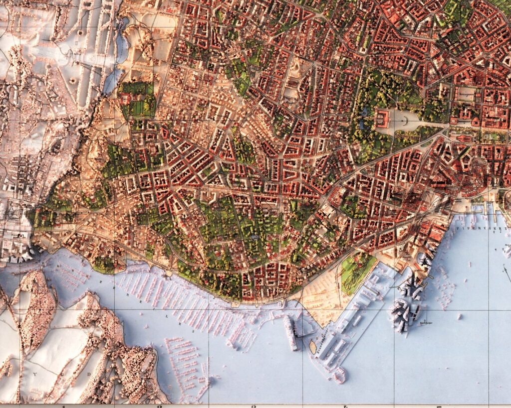
New technology combined with high-resolution elevation data has made possible a new style of terrain maps distinguished mainly by their big, long, dramatic shadows, and their tactile, pop-off-the-page appearance. At Stamen we call this style of cartography “Blender maps”, after the name of the software most people use to make them. This map 1875 map of Switzerland combined with contemporary digital shadows is a prime example of this style:
At Stamen we were immediately inspired and intrigued by this new technique, and set to work thinking about when and how we could use it in our own maps. These Blender maps are undeniably beautiful and cool, but when do they add real value, and when are they just style for style’s sake? How can we make our client projects more effective and eye-catching, without distracting too much from the message in our clients’ data? And what happens if we push these tools to their limits and apply them in unexpected ways? What wild and wonderful new cartographic surprises might we discover?
Later in this blog post, I’ll share some of our experiments with these new shadow-rendering techniques, but first we’ll dig through this deluge of dramatic topography that inspired us. We’ll examine how and why these maps are made, what are they actually good for, and explore where we think this technique could be pushed further.
The ubiquitous “Blender map”
The first time you see one of these maps, the effect is stunning. These maps look more “real” than maps we’re used to seeing, with the hills and mountains seemingly leaping off the screen, with tall peaks casting shadows that stretch across the landscape and sometimes even off the map onto the margins of the page itself. Dark, shadowed valleys evoke a sense of mystery, inviting you to peer into the furrows of the terrain.
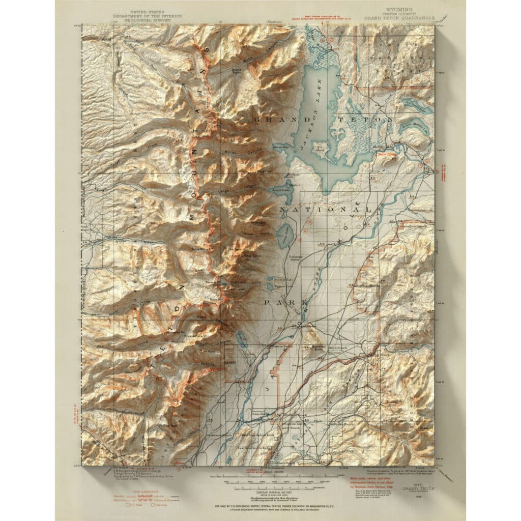
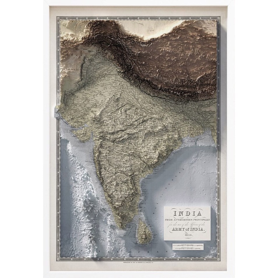
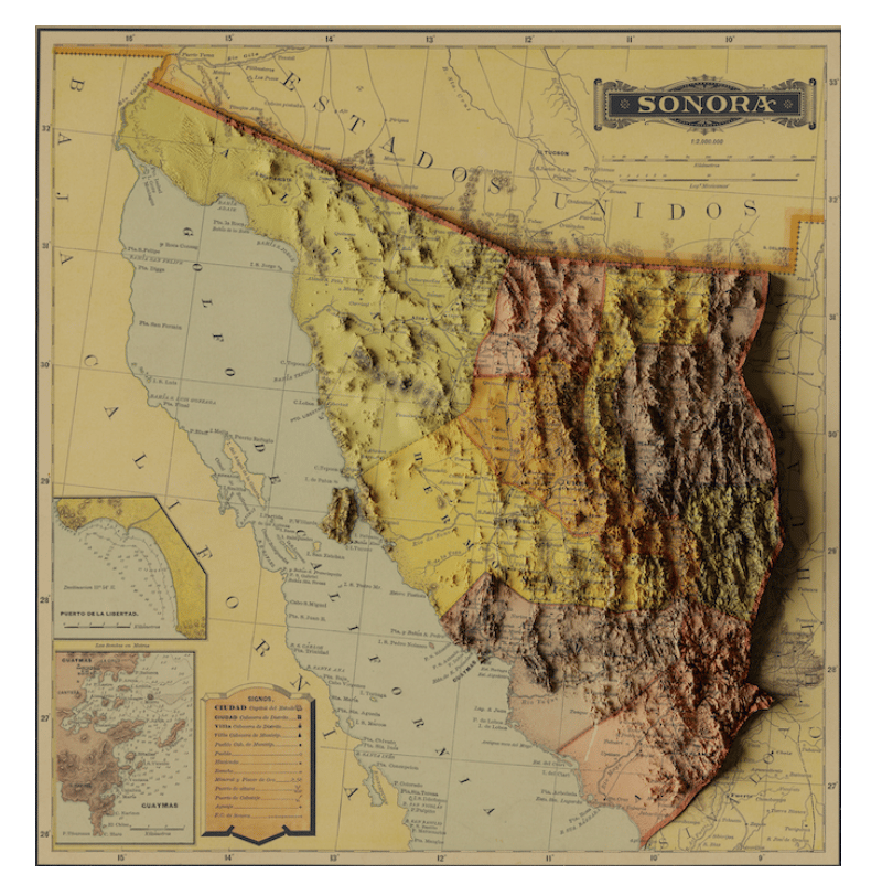
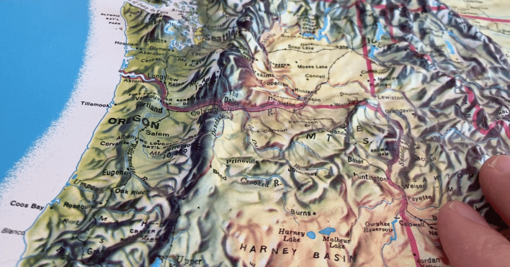
Typically you’ll see a scanned historical map overlaid with richly detailed shadows derived from modern elevation data. The contemporary data is usually derived from high-tech sources like aerial laser ranging (LIDAR) or satellite measurements. This juxtaposition of old and new produces a hyper-real appearance evokes nostalgia for old-fashioned true 3D “raised relief” maps that you might see printed on extruded plastic in classrooms, or hand-carved in park interpretive centers.
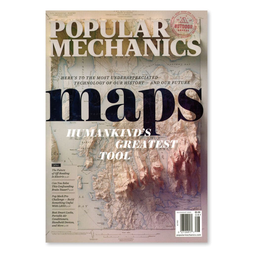
These digitally-rendered Blender shadows were first exposed to a wider audience via Scott Reinhard’s map on the cover in Popular Mechanics’s special issue on maps in July 2020:
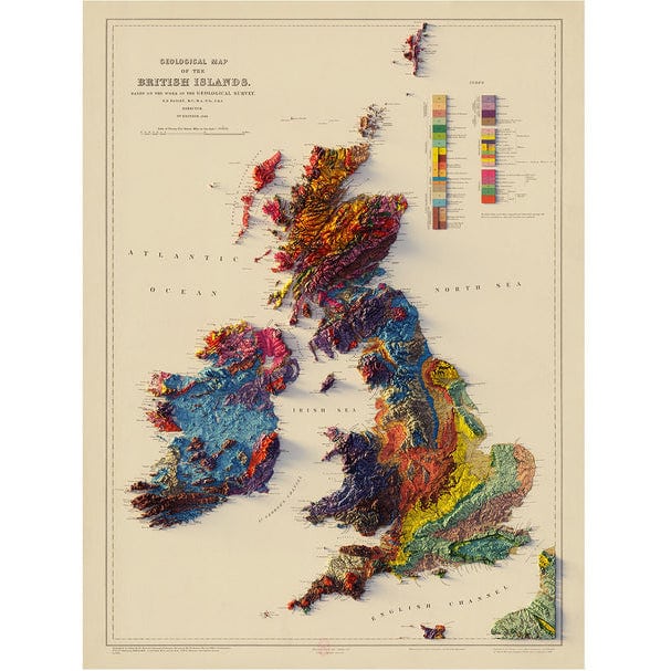
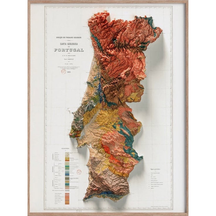
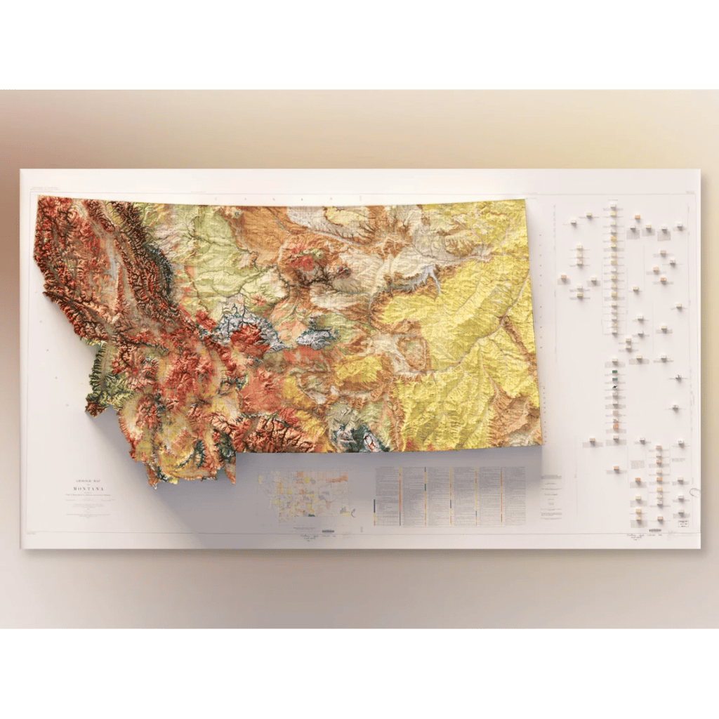
Building on this hyper-real effect, another common style of these maps is to use geological maps with their saturated, otherworldly color palettes.
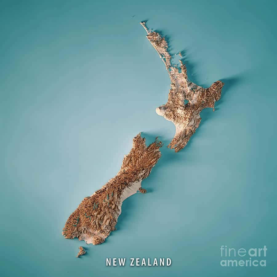
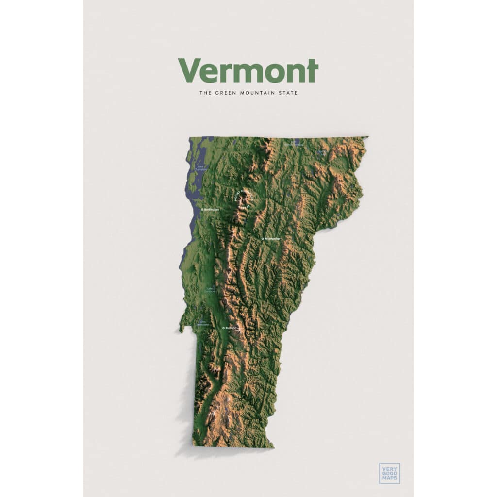
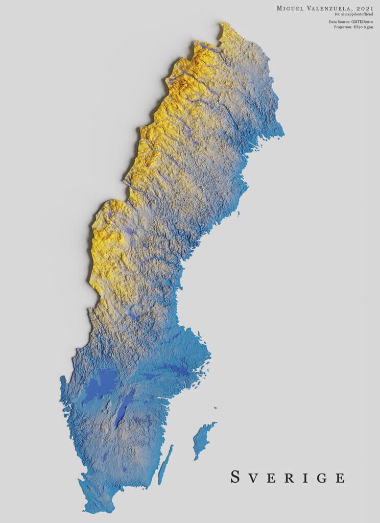
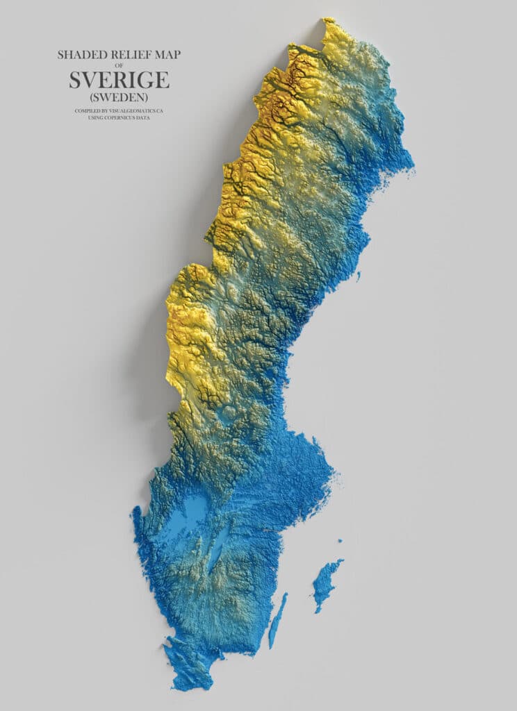
Or for a more minimalist effect, some cartographers stick with just the pure elevation data itself. In these examples, color isn’t derived from an image draped over the terrain, but from a hypsometric spectrum that changes color based on elevation. These color ramps can be relatively monochrome, as in the example below from Frank Ramspott, or sometimes use a green to brown gradient to simulate realistic landcover as in the series by “Very Good Maps”, but they can also can use nearly-psychedelic color spectra as in many examples from 4DMapArt:
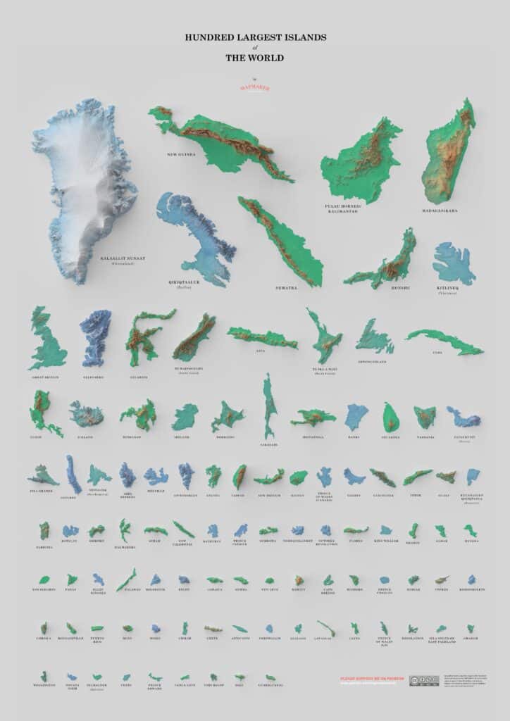
David Garcia’s “Hundred Largest Islands of the World” poster is one of my favorite early examples of this genre, from 2018. I especially like the use of different hypsometric tints to distinguish the arctic islands from temperate and tropical ones:
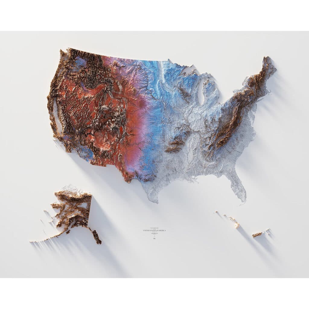
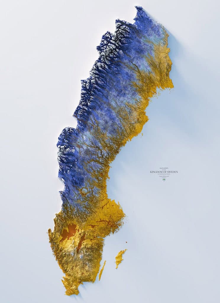
The more we looked at these Blender maps, the more we saw certain techniques repeated again and again. For example, at least three different map makers had the idea of using the colors of countries’ flags as the elevation coloring:
Once we started looking for maps using this technique, we began finding them everywhere. What happened? Why are we seeing all these maps now?
As far as I can tell, this new genre of cartography can trace most of its lineage back to an influential 2017 Blender tutorial written by Daniel Huffman (although map creator Longitude.one credits some 2014 maps created by Lee Griggs using the Maya software as inspiration). Huffman’s detailed and well-written tutorial, called Creating Shaded Relief in Blender, along with the maturity of free software like Blender and the increasing power of desktop computers, means that rich, dramatic shadows are now within the reach of any cartographer.
What’s new about these maps?
To be sure, digital cartographers have been adding shadows to their maps since the earliest days of GIS. What makes all of these new maps so interesting is the different way these shadows are generated. Traditional GIS software renders relief maps with a technique called “hillshading” whereby the terrain at each pixel is examined to see how steep it is relative to the adjacent pixels (the “slope”), and which direction the slope is facing (the “aspect”). Using this information, the GIS can simulate how much light would be shining on that pixel, assuming a point-like light source at a given angle (usually coming from the upper left corner of the screen). But this traditional technique is relatively simplistic, and doesn’t take into account any shadows or reflections caused by pixels anywhere else in the map: it only examines one pixel at a time.

The more elaborate shadows that are now becoming common use a more complex technique called “ray tracing” which simulates the paths of photons coming from a light source (which can be larger than a single point) and models how they bounce off different surfaces and parts of a scene, potentially obscuring or illuminating sides of the landscape that would not have been illuminated or in shadow based on the simpler hillshading technique.
Ray tracing as a technique has been around for a long time, but it is much more computationally intensive, and takes far longer to render, so only in recent years has it become feasible with normal personal computers. Also, new free, open-source software has made these algorithms more accessible to more cartographers.
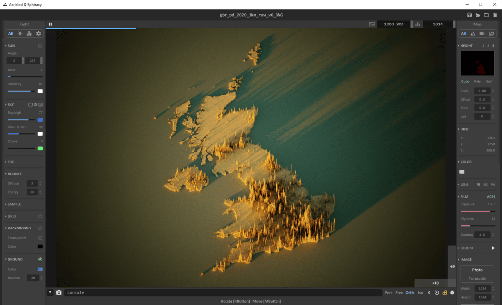
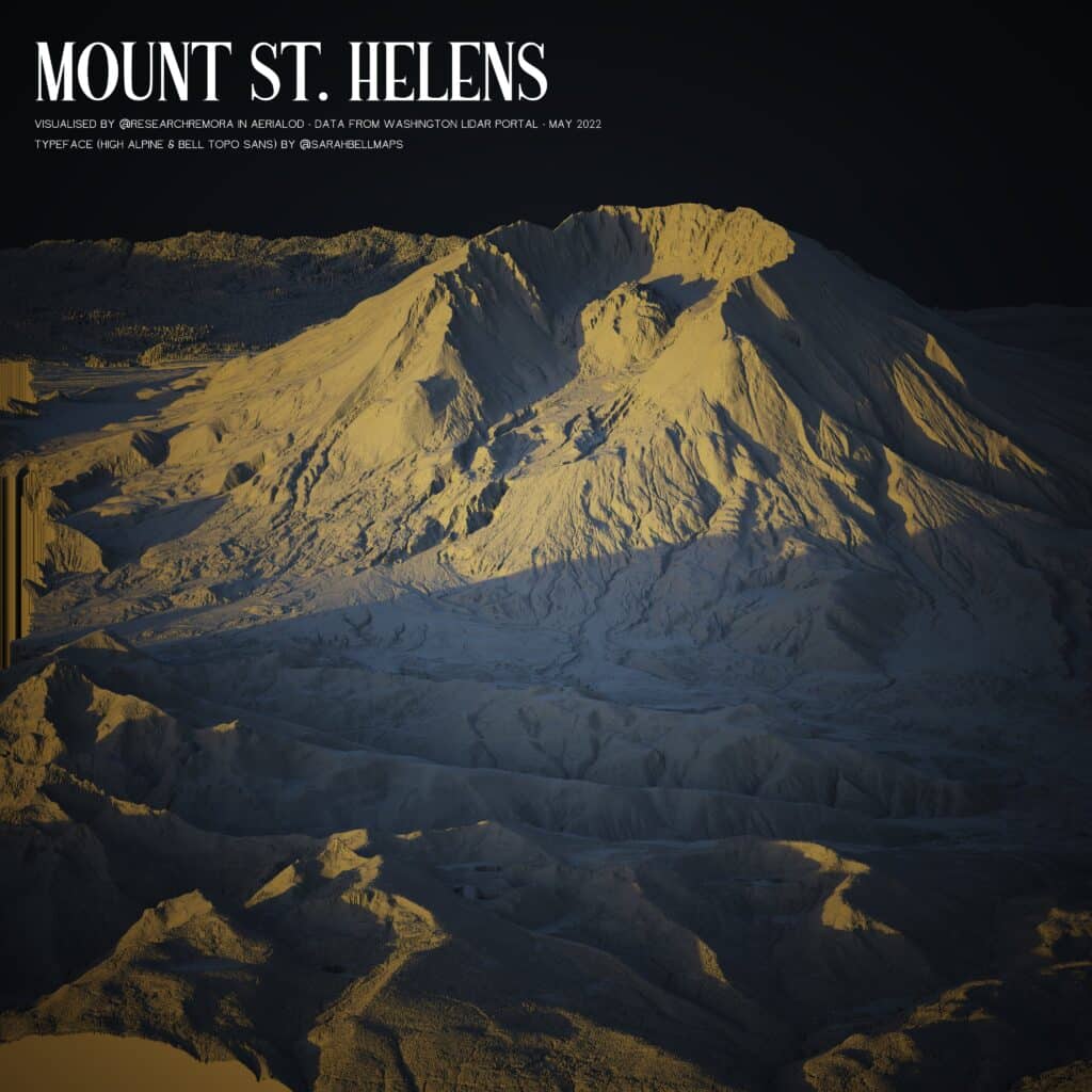
Most of these use a tool called Blender, an extremely powerful open-source tool for all kinds of 3D modeling and rendering. A few cartographers use other tools, such as Aerialod, or R‘s Rayshader plugin.
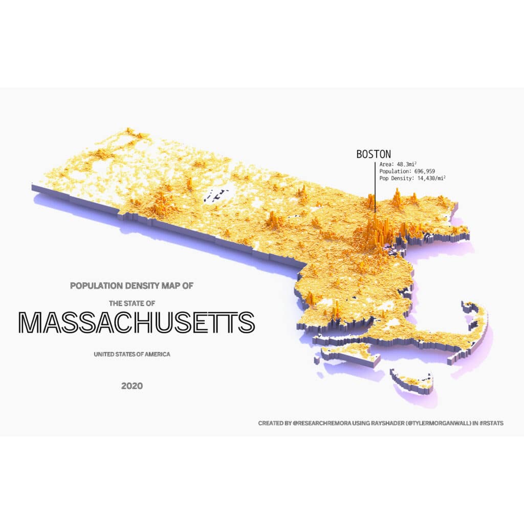
Rayshader, a plugin for the statistics and data analysis software “R”, has a particularly strong online community with copious examples shared on twitter using the hashtag “#rayshader”. The most prolific map maker in the R ecosystem is a twitter user by the name of “@researchremora”.
Moving beyond the “same old Blender maps”
While this young genre has produced a lot of stunning and compelling maps, many of them are already starting to feel the same. The Blender style has already become a trope. Even Daniel Huffman, author of the tutorials that started this trend, is now asking cartographers to “consider making your Blender relief less blender-y.”
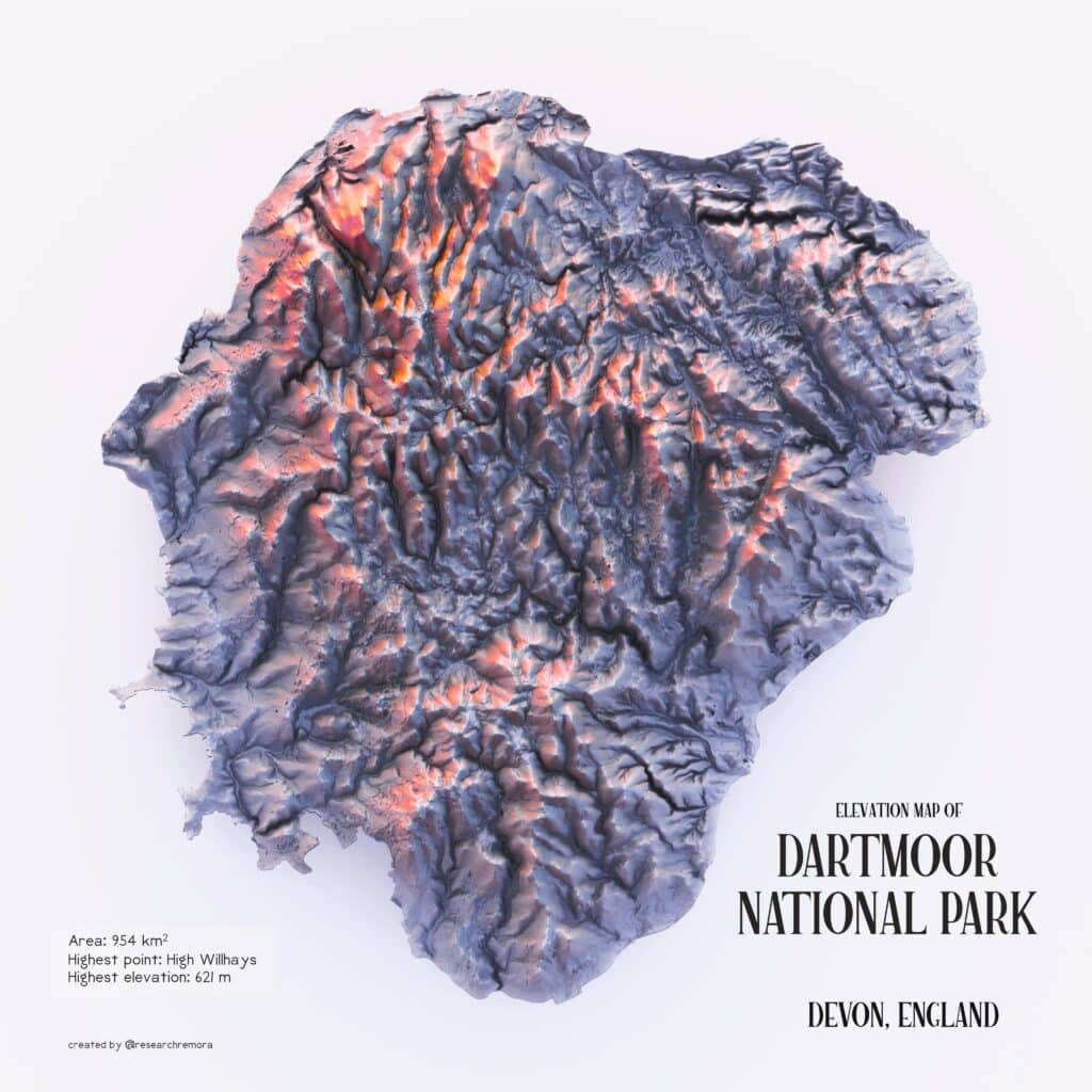
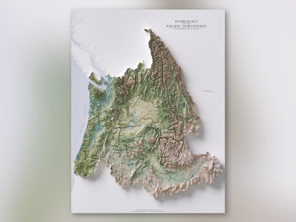
As I sifted through hundreds upon hundreds of Blender maps for this post, I began to appreciate even subtle straying from the typical formula. For example, what if the shaded area is clipped at the edge of a watershed… or at the edge of a national park:
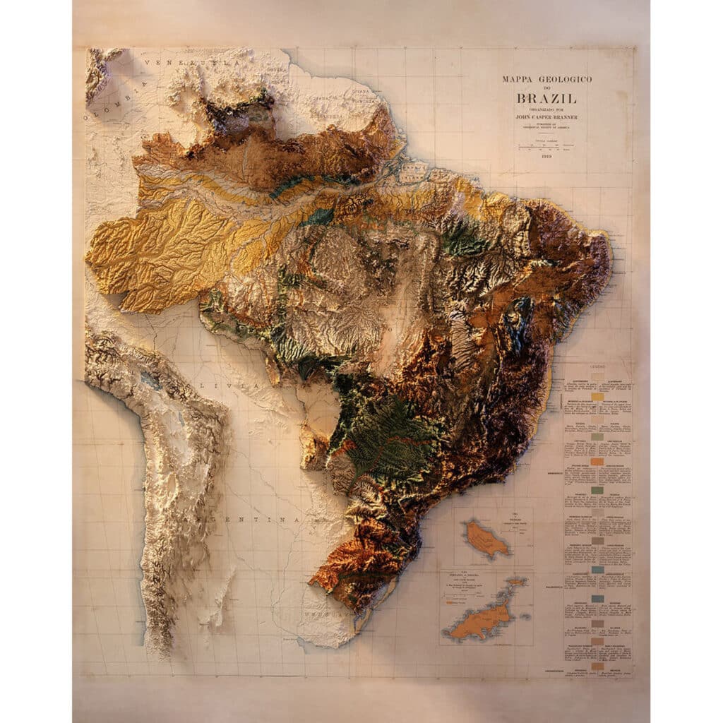
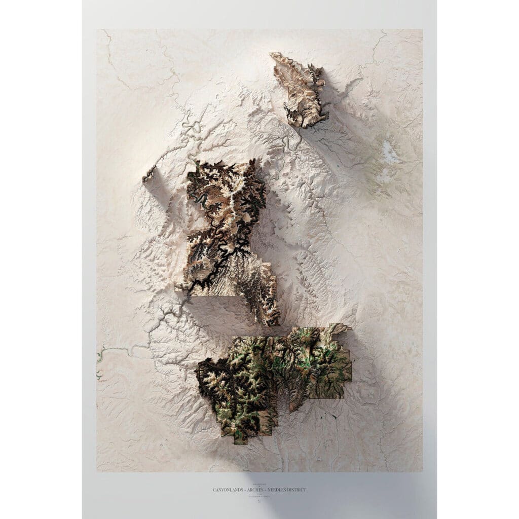
Or what if the relief for the area of interest (say, the borders of a particular country) is exaggerated more than the relief for the surrounding areas? In the example below, note how the mountains of Brazil appear much taller than the Andes mountains visible at the left edge of the page, while in real life the Andes are in fact many tiles taller than any part of Brazil. Or in this example of Arches National Park, observer how the terrain outside the park boundaries is visible, but much less exaggerated than within the park itself:
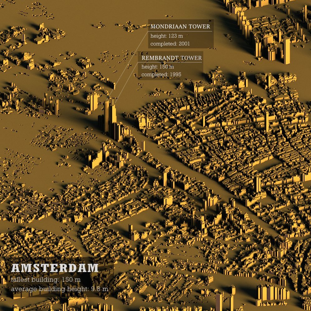
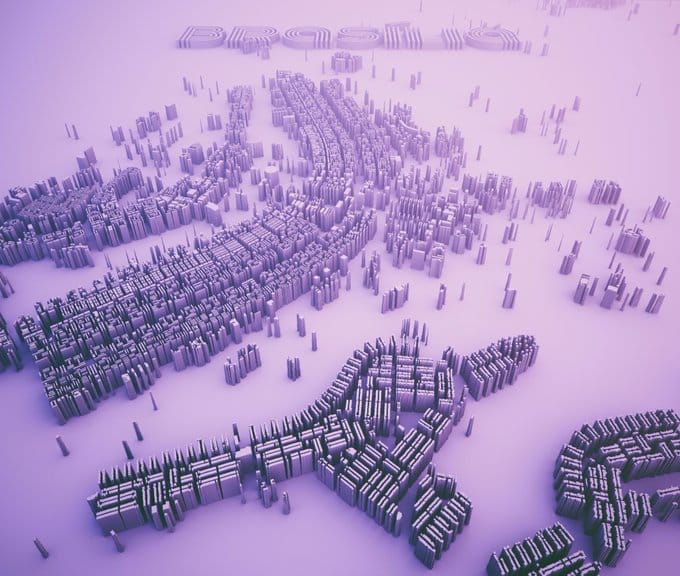
Some cartographers diverge from using terrain data to render building geometries instead. Often these Blender maps that render building data are using building footprint data that includes the height of the buildings, for a fairly realistic impression, but sometimes building footprints used without precise height data, and exaggerated to unnatural proportions, can produce interesting artistic interpretations. And very high resolution LIDAR data of cities often includes buildings, trees, and practically everything else in a cityscape:
Of course there’s no reason why Blender maps have to apply hyper-realistic shadows to real-world things like mountains and buildings. Why not create fictional terrain from other kinds of data?
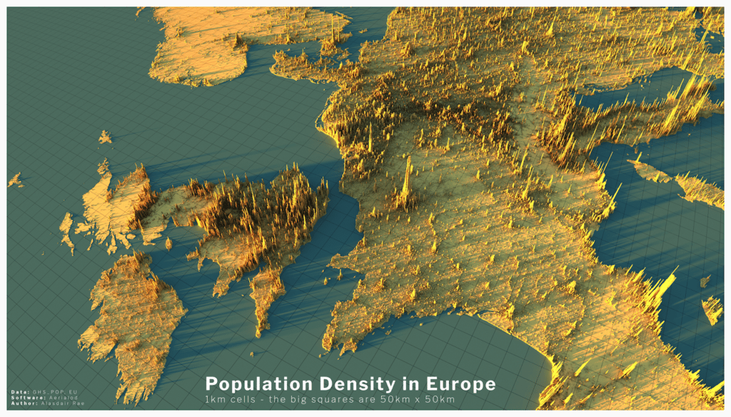
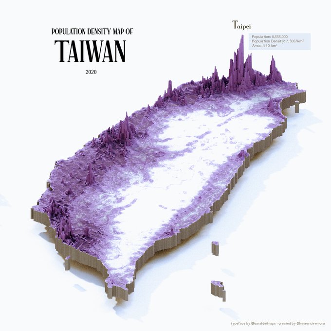
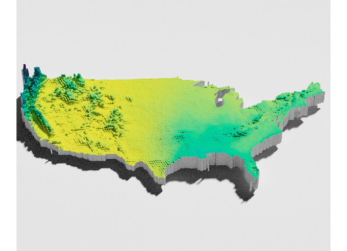
One compelling kind of information to visualize is population data, where the greater the density of people, the higher the peaks on a virtual landscape. Visualizing population density is always a challenge in cartography, because the differences are so dramatic between very dense yet tiny cities, and the wide, low-density rural areas between them. Communicating just how many people live in the city relative to the countryside can be quite difficult in two dimensions, but adding a third dimension, as in these examples from Alasdair Rae, gives a tactile, visceral glimpse of the urban/rural divide:
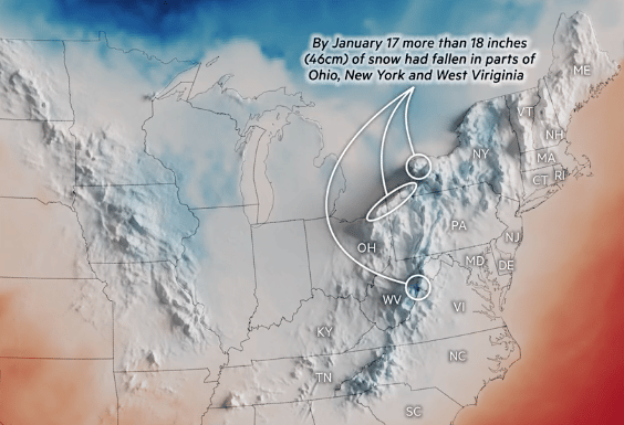
Weather phenomena like rainfall or snow accumulations also make for fascinating terrain:
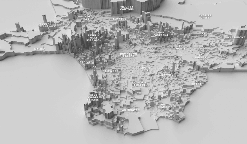
Nick Underwood’s visualization “The Topography of Wealth in L.A.” includes a stunning 3D fly-through of Blender-shaded terrain representing the household income in each census tract in Los Angeles County:
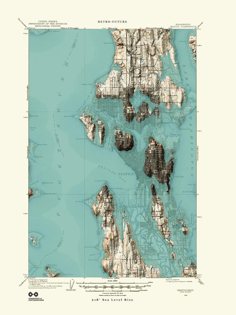
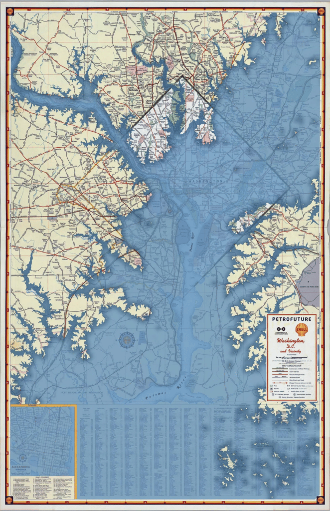
Finally, I’d like to highlight at least one cartographer who is sticking with the original trope of Blender hillshades plus scanned historical maps, but manages to deliver an important message by altering the source data itself: in his series of “retrofuture” and “petrofuture” maps, Jeffrey Linn combines historical topographic maps and gas station travel maps with terrain where sea level has been recalibrated to show the effects of melting ice caps:
Where next for Blender terrain?
In this survey of the, ahem, “terrain” of Blender cartography, it’s heartening to see these examples of people pushing the boundaries of what is possible with these new tools and techniques. But there are at least three aspects of these maps that I think could be explored further. Here are a few quick experiments illustrating where Blender maps might go from here:
They’re all just… “shadows”
First of all, in cartographer-speak, these are all “univariate” maps. That is, the size of the shadows only communicates one variable at a time, whether that’s elevation, population, precipitation, etc. They all only need a grayscale color ramp to communicate information, no color is needed. But at Stamen we are always looking for opportunities to use color mixing to communicate more than one variable simultaneously.
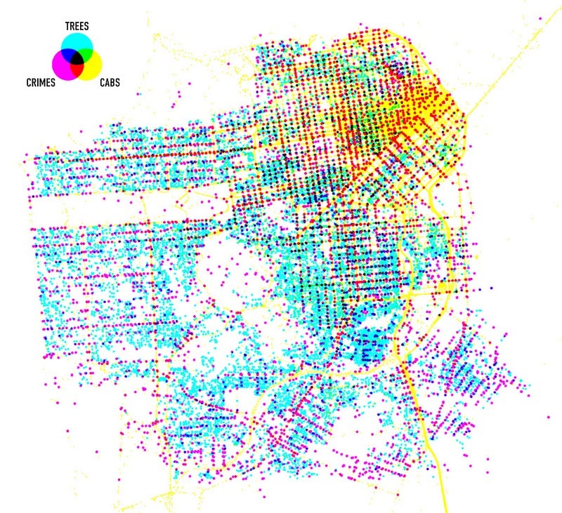
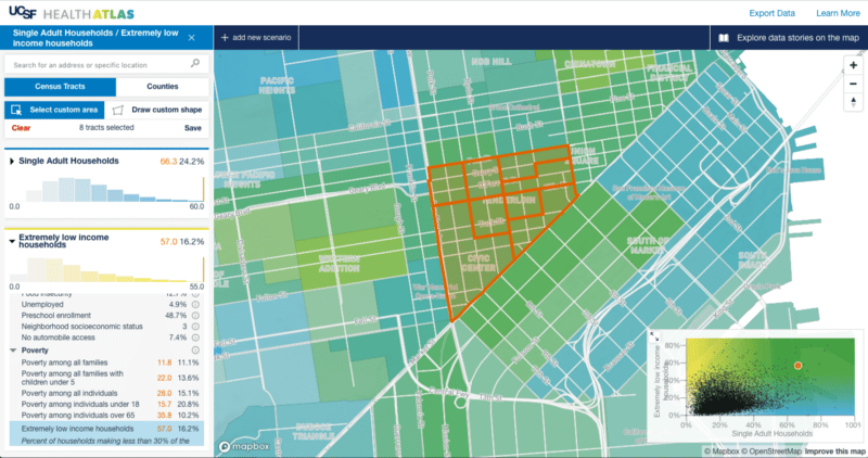
To explain what I mean by bivariate or multivariate mapping, let’s look at some examples (and you can also read more in one of our previous blog posts by Curran Kelleher). One of my favorite Stamen projects (from before my time) is the Trees, Cabs, and Crime map made by Shawn Allen in 2012, where three variables are mapped using cyan, magenta, and yellow, and the overlaps between them blend to create additional colors. More recently we used a bivariate color scheme as part of a dynamic choropleth map for the UCSF Health Atlas. Each census tract is tinted from white to yellow according to one variable, and also from white to blue to show a second variable (resulting in a blended green where the values for both variables are high).
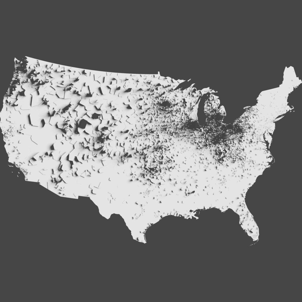
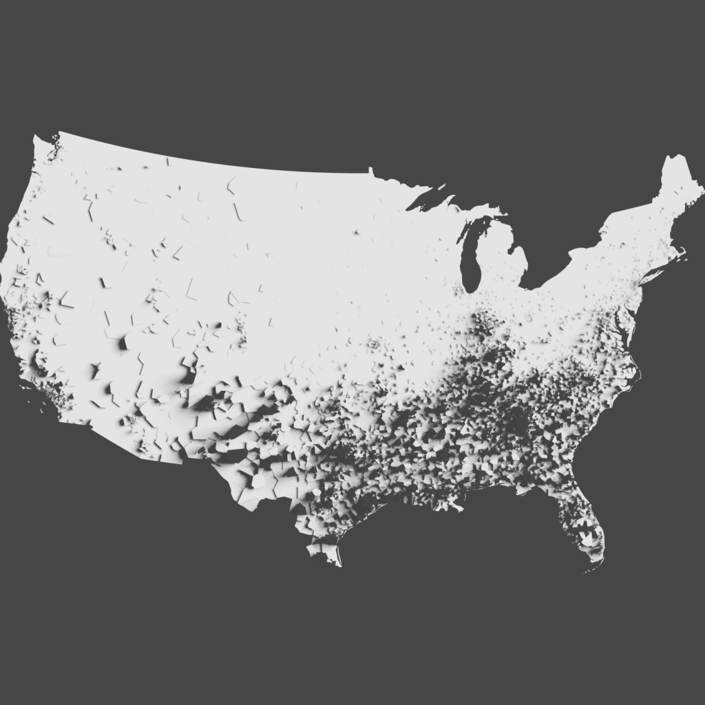
If we bring this multivariate color-mixing mindset to the world of Blender, what would happen if there were multiple shadows in different colors cast by different datasets? In this experiment I create three separate univariate maps, using data derived from the Pop vs Soda survey. I used the number of survey responses in each zip code in the US to create a virtual terrain, first for “soda” responses (mostly in the Northeast and in California), then for “pop” (mostly the Midwest), then finally for respondents who said “coke” (primarily in the South).
With those three sets of shadows colorized in Photoshop and then blended together, perhaps we can see where the different overlapping of shadows mix to produce new colors in the spectrum, producing combined green shadows in the Northwest where both “pop” and “soda” are common terms, or mixed bluish-purple areas in places like North Carolina where both “coke” and “soda” are common.
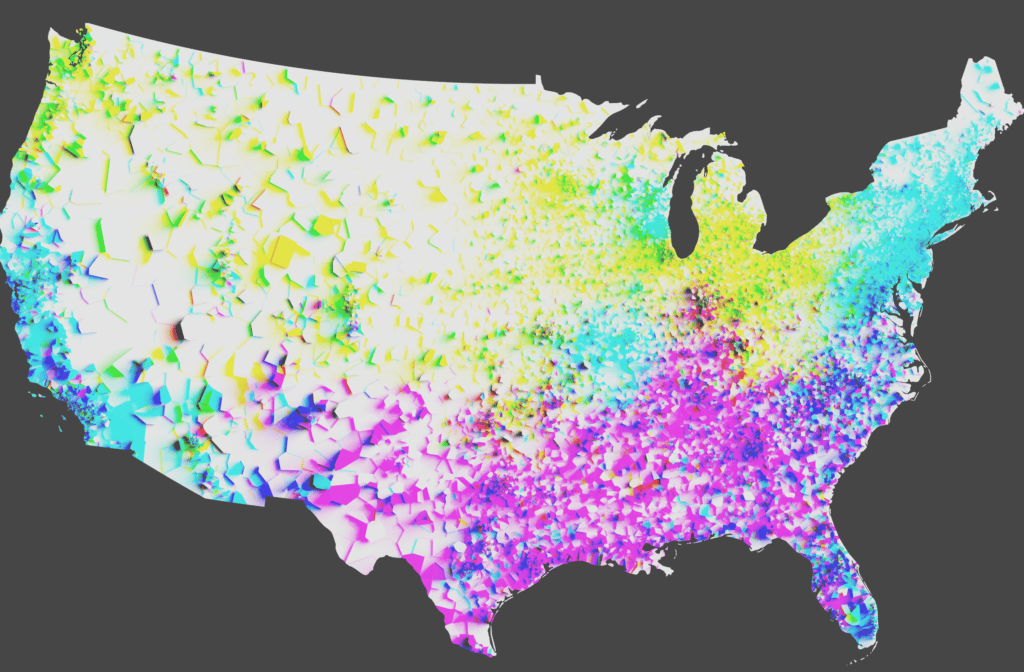
Does it “work”? As a quick experiment, it’s intriguing, but I think the technique could use a lot more refinement.
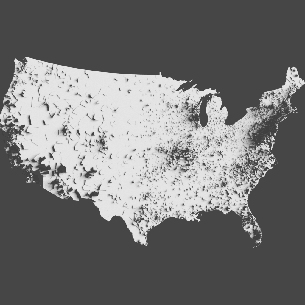
As a second experiment in this vein, I tried the same concept but with county-level data from the 2020 presidential election. I was interested in seeing if this technique could break out of the conventional thinking about blue cities and red rural areas (a cartographic challenge I talked about a lot in my 2020 election map roundup post). While it is true that rural areas do usually vote more for Republicans than Democrats, the bulk of Republican votes (in terms of raw numbers) usually are found in cities and suburban areas too. In a Blender map, cities would cast a long blue shadow, but they would all cast a fairly significant red shadow too.
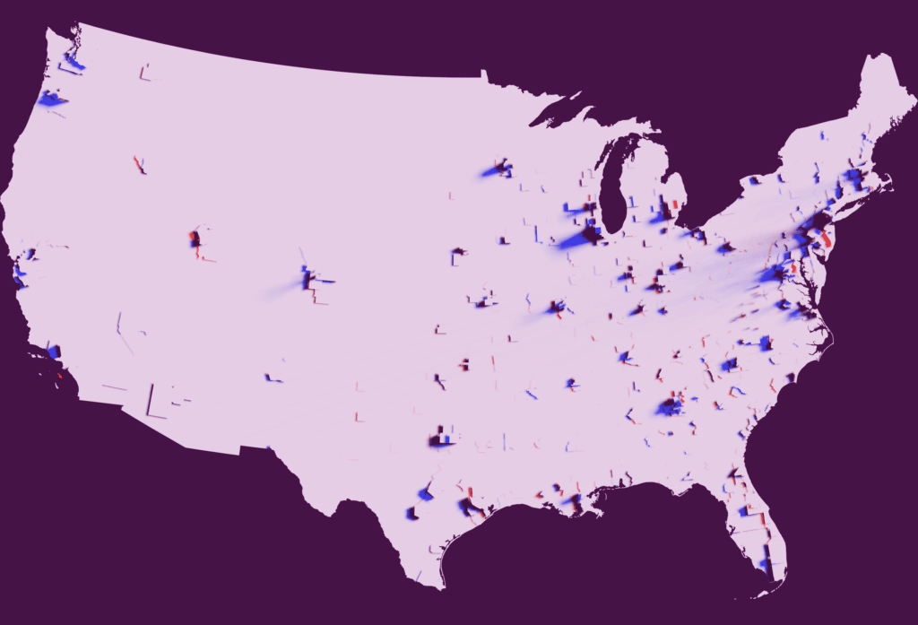
Again, does this quick map tell that story well? Maybe… if you look closely you can see metro areas like Dallas and Salt Lake City where the urban shadow is almost black, suggesting that the votes in those areas are almost balanced by party, whereas in more strongly democratic cities like Chicago, you can see how the blue shadow far outstretches the red one. Again, I’d like to experiment with this technique more, and I’d encourage other cartographers to give this a try as well. Let me know if it works for you!
Maybe just shadows on a few things...
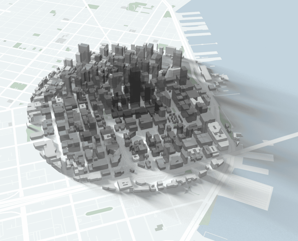
Another thing we noticed about all of these Blender maps is that none of them use the zoomable tiled web maps that we are familiar with for interactive online maps. There are some big challenges with making a tiled version of a Blender map (which I’ll explore below) but one way to short-circuit those problems is to selectively apply the shadows only to a very limited area. We’ve done this in the past, using shadows just to highlight a few features, which is something that’s feasible in a tiled web map by creating the shadow image in Blender and then loading that image as a tiled overlay in a Mapbox map. This technique works particularly well for giving more depth and realism to some selected buildings, but might not be quite as effective for terrain visualization.
Creating truly interactive and dynamic shadows (where the light source changes as you interact with the map) is still very difficult to achieve. Blender can take several minutes to calculate shadows for a complex model such as the downtown San Francisco buildings in this example, far too slow to be interactive. But by pre-rendering the shadows for a selected area and inserting them into a map where everything else is interactive–the zoom, pitch, and angle of the map, and even whether or not the building shapes themselves are displayed–we can bring a “good enough” hillshade experience into a the interactive maps that users have come to expect on the web.
They’re all static…
Finally, as I mentioned above the most striking thing missing in my survey of Blender maps is that you never see these types of shadows on an interactive zoomable/pannable map (a “slippy map” in cartography lingo). Why is that?
The problem is this: the reason “slippy maps” work so efficiently is because every tile has been pre-generated, and that each tile only contains data within its narrow bounding box. This means that a slippy map can quickly stitch together multiple tiles to fill your browser window with a map of any size and proportions, but only because the contents of each tile are effectively unaware of the contents of their neighbors.
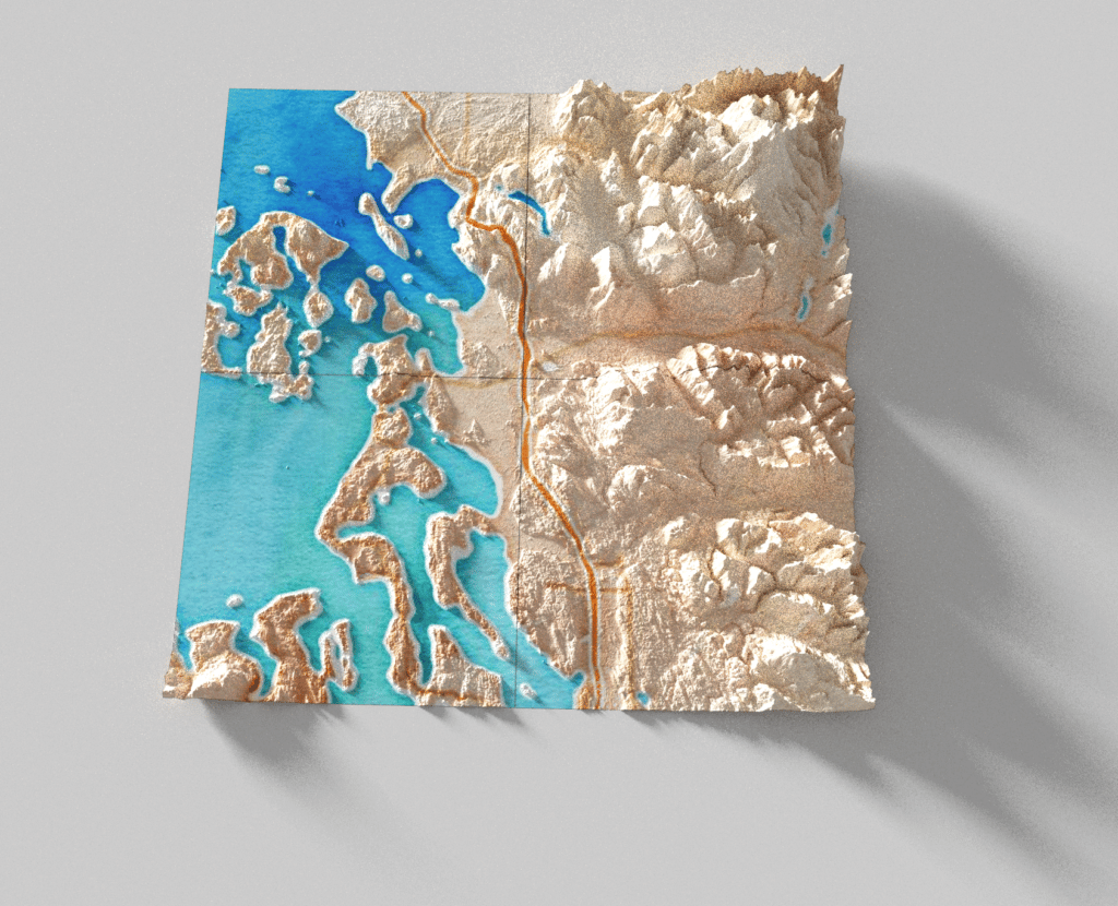
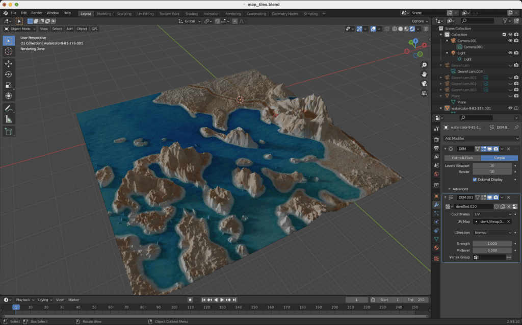
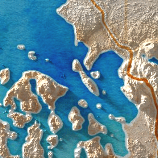
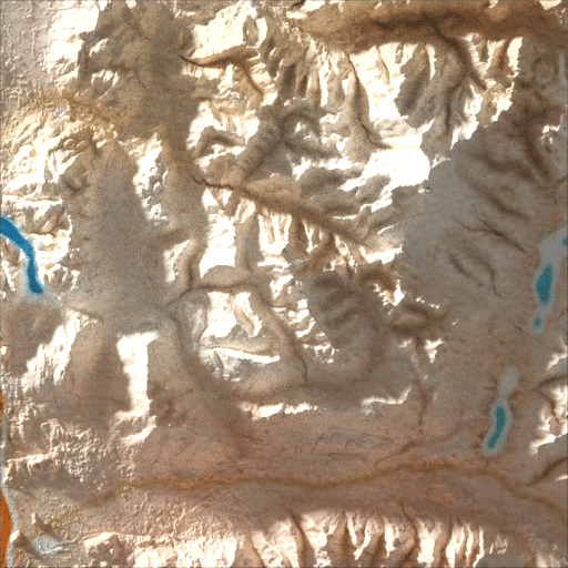
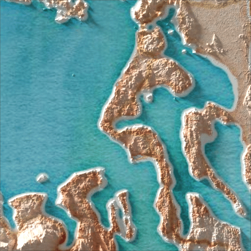
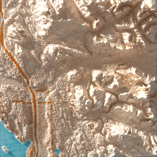
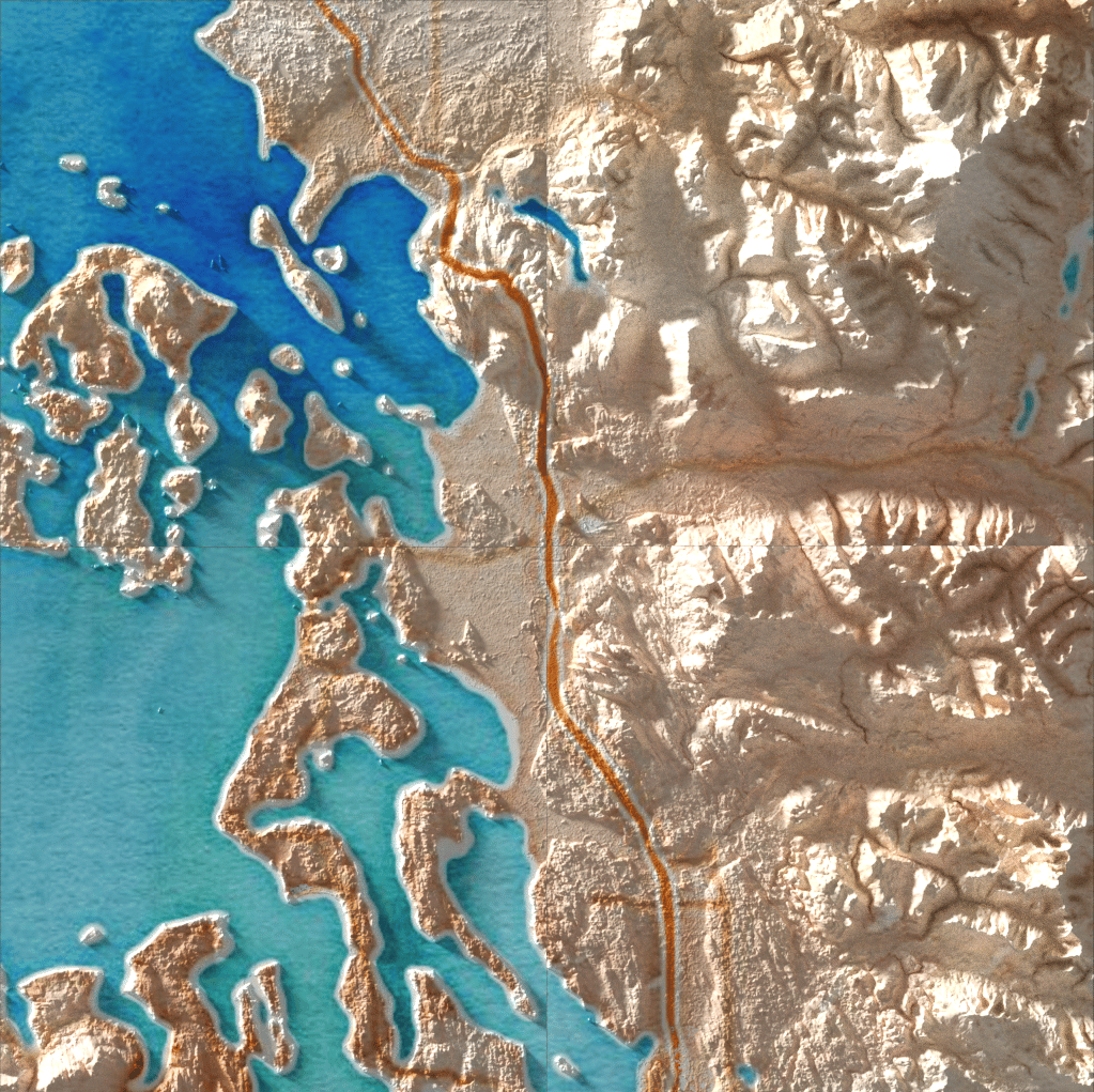
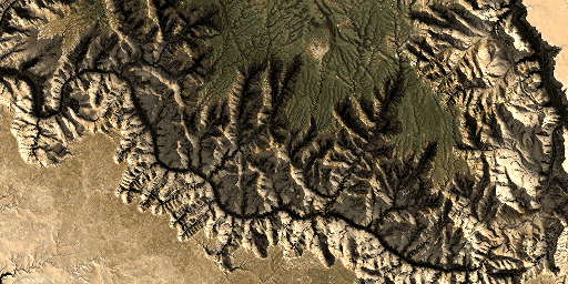
So what if we tried to apply Blender hillshades to a few slippy map raster tiles (these ones are Stamen Watercolor tiles from zoom 9 in an area around Bellingham, Washington). We can see that the dramatic shadows from the terrain in each tile would need to spill out onto the neighboring tiles.
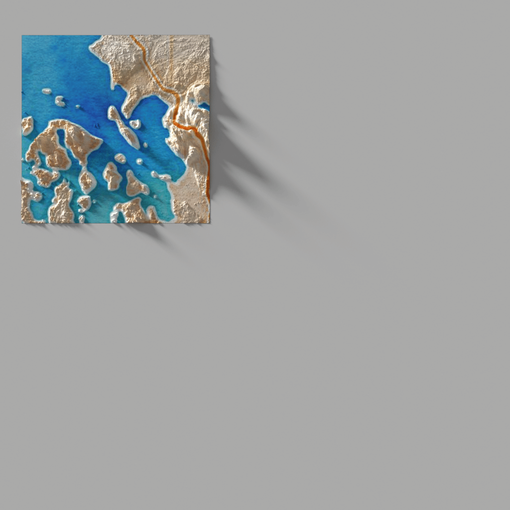
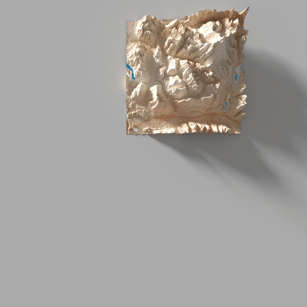
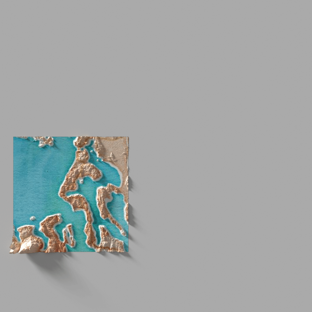
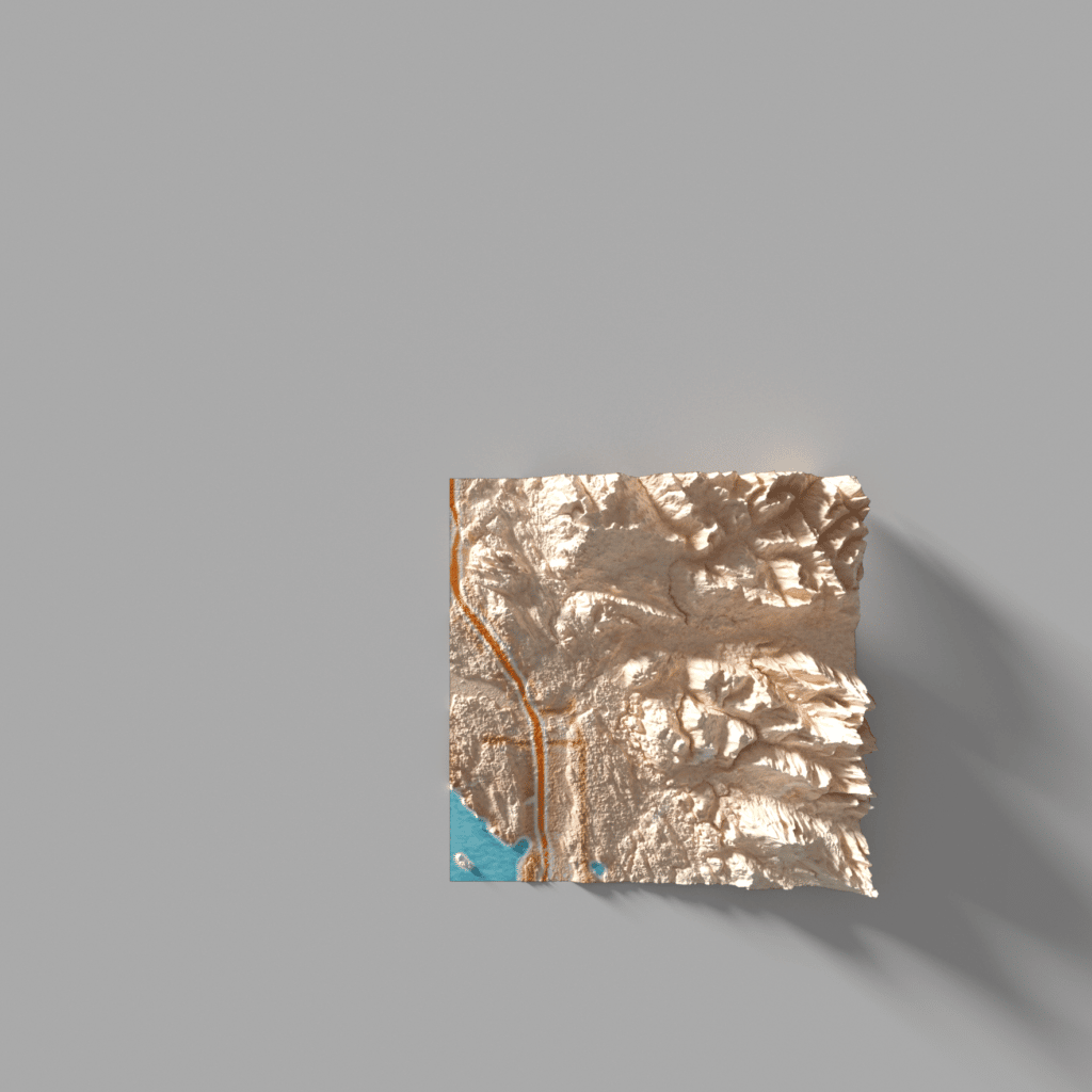
But if we sliced up those tiles just to their exact bounding boxes (as required by the way slippy maps work) we can see that each tile is unaware of the shadows that the neighboring tile should be casting upon it.
Stitching them together (as in a tiled web map in your browser) the result is pretty good, but you can see some weird-looking shadows at the tile boundaries. This approach wouldn’t work for a global tiled web map.
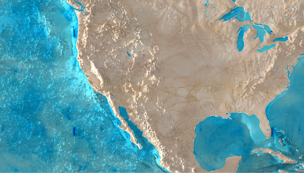
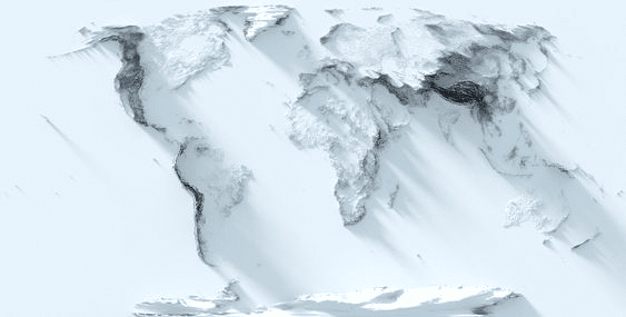
If we stick to a very zoomed-out map, or if we have a really huge computer running Blender, we could try to do a hillshade for the entire world, and then slice that up for our map tiles. But there’s no way we could do this at a high-enough resolution so you could zoom all the way in, as in the sample tiles above.
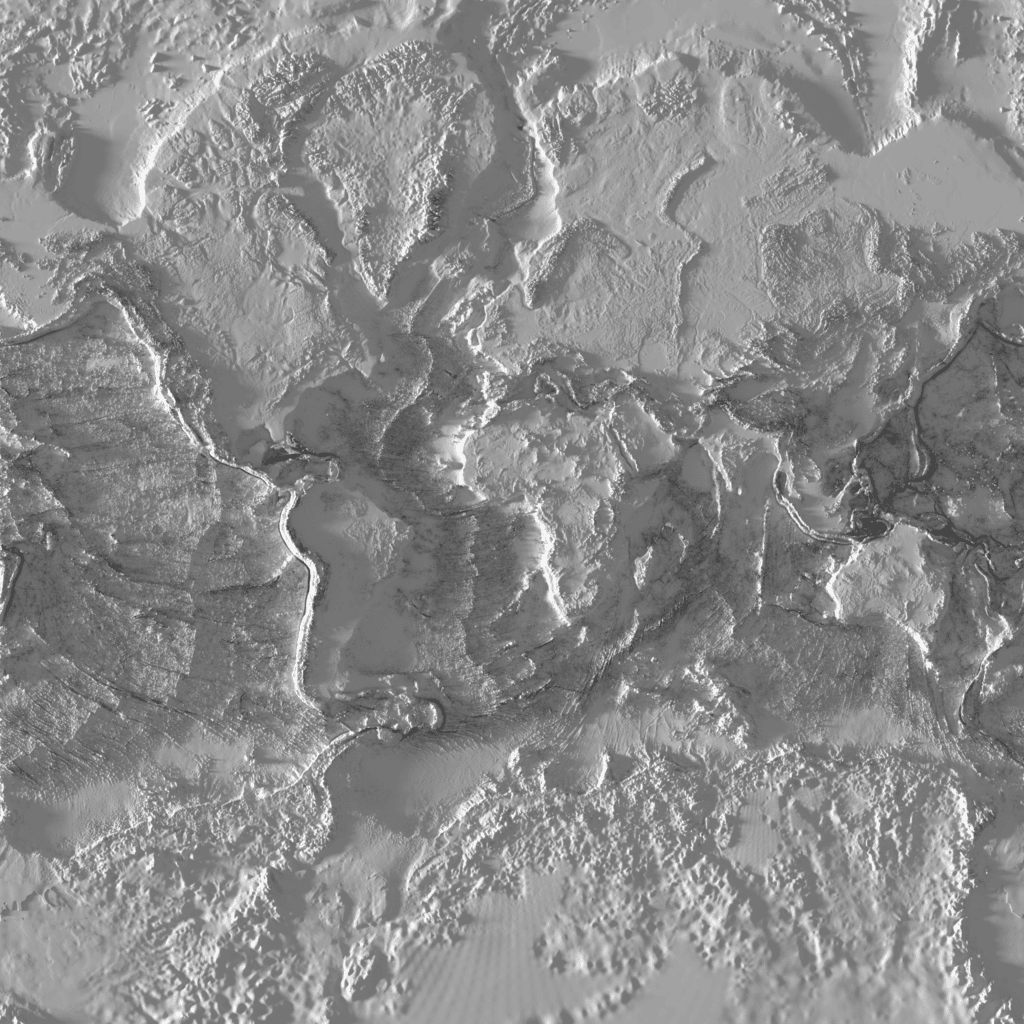
Above: a Blender hillshade for the whole world, suitable for up to zoom 5 or 6. The end result might look like this, but you wouldn’t be able to zoom in any further:
We have some ideas about how we could work around these problems, and make a truly world-wide high-resolution Blender-style hillshade for map tiles, but it would take a bit more work. Some very impressive ground work creating rayshaded shadows for map tiles can be found in the “Advanced Map Shading” blog post by Rye Terrell, including some of examples of the necessary buffering you’d need to do in order to accurately calculate the shadows cast by neighboring tiles:
Nobody has made world-wide high-resolution Blender-style hillshade for a tiled web map (yet!) but now it should be possible, if the right project calls for it. If you’re interested in collaborating with Stamen or hiring us to make such a map, give us a call!
What did I learn?
It’s not easy
While it’s true that “anyone can make these maps” these days, I don’t mean to imply it’s easy! I can guarantee that every one of the Blender cartographers featured above has spend days, weeks, and months learning how to use these tools, painstakingly cleaning up their source data, and carefully tweaking countless settings to get an output that looks good. When trying to make my own Blender hillshades, I was surprised how complex, unfamiliar, and unforgiving the Blender interface is! As is often the case with powerful open-source tools, people keep adding settings and creating interfaces that make sense for the power-users who request them, but drift further and further from usability focused on beginner or intermediate users. Blender’s steep learning curve means that cartographers need quite a bit of determination to make their own maps using these techniques.
Will there be any “drag and drop” settings in future tools, where you can load your data into a GIS program or graphic design software and click an “add hillshade” button? Something like that might be possible, but if that happens, brace yourself for an even greater deluge of Blender-style maps and even more homogeneity of what they look like.
And what about the experiments I shared above? This post isn’t meant to be a tutorial (see Huffman for that), but I may follow up with some more technical specifics about some of the experiments I created in my journey of exploring the world of Blender. Don’t hesitate to get in touch if you have questions about how I made any of the examples at the end of the post!
Does it really aid understanding? Probably… not?
I hope you didn’t need to read any labels in those shadowed valleys in Switzerland, which is where most people actually live! The more we dial up the drama in these Blender hillshades, the more those steep valleys become almost black in the final render. If you think your map reader needs to see down into those valleys, you probably should rethink the boldness of your hillshade.
The hyperreal-effect also risks being interpreted as reality: but seriously, standing in Kansas City nobody’s ever had the sun blocked out by the Rocky Mountains. Surely as cartographers and designers we think to ourselves that no one will mistake these maps for reality, but can you really be so sure? Especially with some of these other examples above that are not so clearly abstractions?
When taken too far, these shadows cross the line into becoming like Edward Tufte’s “chart junk”. If the map becomes more about the shadows than the content of the map itself, is that want we really want?
“Occasionally designers seem to seek credit merely for possessing a new technology, rather than using it to make better designs. […] But at least a few computer graphics only evoke the response “Isn’t it remarkable that the computer can be programmed to draw like that?” instead of “My, what interesting data.”
Edward Tufte, The Visual Display of Quantitative Information (1983)

But that’s okay!
If we keep in mind what these maps are for, (and the purpose of each of these maps is as unique as the maps themselves) we can evaluate whether these shadows are successful. And for maps that are meant to be a think of beauty, they succeed. And to be clear, there is absolutely nothing wrong with that!
It makes me think of a quote often used by Stamen founder Eric Rodenbeck when talking about our Watercolor map style: “These are maps for dawdling, not for navigation”. The same is true more or less for Blender maps. If you are looking for a map that is utterly true to the data and single-mindedly focused on helping users achieve a concrete task, these are not the maps for you! But if you want to make a map that invites readers to pause, explore, and appreciate a moment of beauty, then using Blender in your cartography workflow might lead you to the right place.
At Stamen we’re still thinking about how to gracefully and impactfully incorporate Blender-style shadows in our workflows in ways that will serve the needs of our clients and their users. If you have any ideas about how our cartographers can help you and your business, please get in touch with us!